Computing the eigensystem#
So far we have focused on individual eigenvalues and eigenvectors. Now we turn to the QR iteration, which builds on the QR decomposition/factorisation we studied earlier.
The Schur decomposition#
The eigenvalue decomposition \(A = X\Lambda X^{-1}\) is not always suitable for computational purposes. It might not exist, requiring a Jordan normal form instead. Even though small machine perturbations usually ensure diagonalizability in floating-point arithmetic, the proximity to a Jordan form can introduce instabilities. The eigenvector matrix \(X\) might also be ill-conditioned, making its inverse computationally unreliable.
For practical computations, the Schur decomposition of \(A\) is more robust.
Theorem 18 (Existence of the Schur decomposition)
Every complex matrix \(A \in \mathbb{C}^{n \times n}\) has a Schur decomposition
with unitary \(Q\in\mathbb{C}^{n\times n}\) and upper triangular \(R\in\mathbb{C}^{n\times n}\).
The proof is given in the optional material section below. Let us note some key properties of the Schur decomposition:
Eigenvalues: The eigenvalues of \(A\) are the diagonal elements of \(R\). This is evident from the equation \(\det(\lambda I - A) = \det Q \det Q^H \det(\lambda I - R)\) and expanding the determinant of \(\lambda I - R\) along its diagonal.
Hermitian Matrices: For Hermitian \(A\), the Schur decomposition coincides with the eigenvalue decomposition. Since \(A = A^H\), it follows that \(R = R^H\), so \(R\) is diagonal. The columns of \(Q\) are then orthonormal eigenvectors of \(A\).
Invariant Subspaces: Consider \(R_k\), the upper left \(k \times k\) principal submatrix of \(R\), and \(Q_k \in \mathbb{C}^{n \times k}\), the matrix of the first \(k\) columns of \(Q\). It holds that \(AQ_k = Q_kR_k\). This implies that for any vector \(v\) in the span of \(\{q_1, \ldots, q_k\}\), \(Av\) is also in this span:
\[ v\in \text{span}\{q_1, \dots, q_k\} \implies Av\in \text{span}\{q_1, \dots, q_k\}. \]We say that the subspace is invariant under \(A\). The Schur decomposition thus reveals a sequence of enlarging invariant subspaces.
Pure QR iteration#
In its basic form, the QR iteration is surprisingly simple.
Algorithm 5 (Pure QR iteration)
Inputs \(A \in \mathbb{R}^{n \times n}\)
Outputs \(\{A_k\}_{k\in\mathbb{N}} \subset \mathbb{R}^{n\times n}\), \(\{Q_k\}_{k\in\mathbb{N}} \subset \mathbb{R}^{n\times n}\), \(\{R_k\}_{k\in\mathbb{N}} \subset \mathbb{R}^{n\times n}\)
\(A_0 := A\).
For \(k \in \mathbb{N} \setminus \{0\}\):
Compute QR factorisation of \(A_{k-1}\): \(Q_k \, R_k = A_{k-1}\)
\(A_k = R_k \, Q_k\)
The first observation is that all \(A_k\) are similar:
and therefore
Hence, the QR iteration returns the above Schur decomposition if
where the convergence may be (by norm equivalence) understood in any matrix norm \(\| \cdot \|\).
Theorem 19 (Convergence of the pure QR iteration)
Let \(A \in \mathbb{R}^{n \times n}\) be non-singular and diagonalisable with eigenvalues of distinct moduli:
Suppose that the inverse of the matrix \(T = (v_1| \ldots| v_n) \in \mathbb{R}^{n \times n}\) of normalised eigenvectors \(v_k\) of \(\lambda_k\) has an LU decomposition without pivoting (i.e. \(T^{-1} = LU\)). Then, with signs adjusted as necessary, the \(A_k\) converge linearly to \(R\):
Proof. For the full proof see [Plato, 2003] or [Trefethen and Bau, 1997]. Here we cover the convergence of \(A_k \to R\) in the simpler case \(n = 2\) without determining the rate of convergence.
We conclude from the above that
Let \(q_k\) be the first column of \(Q_1 \cdots Q_k\). Then the previous identity gives
This is exactly the defining equation of the power iteration, with that top-left entry \((R_{k+1})_{11}\) taking the role of \(\lambda^{(k)} = (q_k)^H A q_k = (R_{k+1})_{11} \| q_{k+1} \|^2 = (R_{k+1})_{11}\). As the hypotheses of the theorem include those needed for the convergence proof of the power iteration, \((R_{k+1})_{11} \to \lambda_1\) and \(q_k \to v_1\) as \(k \to \infty\).
In the case \(n = 2\), once the first column of \(Q_1 \cdots Q_k\) has converged, the second column is determined up to sign by orthogonality. Hence, after adjusting signs if necessary, the products \(Q_1 \cdots Q_k\) converge to an orthogonal matrix \(Q\). Finally,
Practical QR iteration#
In practice, the QR iteration is modified to increase the rate of convergence.
The first is to build in the idea of shifts, that we have already come across as \(\sigma\) when studying the inverse iteration.
The second is to transform the matrix first into a similar Hessenberg matrix; in the symmetric case this reduces to a tridiagonal matrix.
In addition, techniques can be applied to break the iteration into smaller (computationally cheaper) subproblems when zeros in off-diagonal entries are discovered. These approaches are called deflation strategies.
For real symmetric matrices the resulting QR iteration is very efficient and requires only \(\mathcal{O}(n^3)\) operations to reach machine accuracy.
Numerical investigation of QR iteration steps#
We investigate these techniques by means of a computational example.
import numpy as np
from scipy.linalg import qr, hessenberg
from matplotlib import pyplot as plt
We start with some random matrix \(A\).
rand = np.random.RandomState(0)
n = 10
A  = rand.randn(n, n) + 1j * rand.randn(n, n)
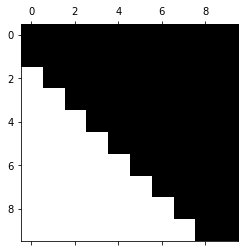
Let us first transform the matrix to upper Hessenberg form. This can be implemented as a similarity transformation that does not change the eigenvalues.
H = hessenberg(A)
plt.spy(H)

We see that the matrix and its first subdiagonal are both non-zero. Upper Hessenberg structures are preserved by a QR iteration step. Let’s check this.
Q, R = qr(H)
H2 = R @ Q
plt.spy(H2)
This structure preservation can be used to implement a QR iteration step in a highly efficient manner. We will not go into technical details about this here.
Let us now run a couple of iterations of the QR iteration and let’s see how quickly the second-to-last element in the last row of \(H\) converges to zero. If that subdiagonal element is zero, then the bottom-right diagonal entry is an eigenvalue (you can verify this by considering the block structure).
nsteps = 300

H = hessenberg(A)

residuals = np.empty(nsteps, dtype='float64')

for index in range(nsteps):
    Q, R = qr(H)
    H = R @ Q
    residuals[index] = np.abs(H[-1, -2]) / np.abs(H[-1, -1])

plt.semilogy(residuals)
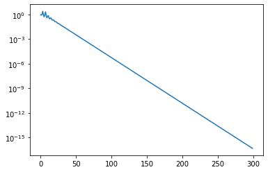
The convergence is extremely slow. We can accelerate convergence using a shift strategy. This modifies the QR iteration step to the following form
Hence, we subtract the shift, compute the QR decomposition, and then add the shift back after forming \(R_mQ_m\).
One can show that a QR step is equivalent to inverse iteration applied to the last vector in the simultaneous iteration. Hence, by applying the shift we perform a shifted inverse iteration. What shall we use as shift?
It turns out that we achieve quadratic convergence if we simply use the bottom right element of the Hessenberg matrix in each step as shift. This is similar to the Rayleigh quotient method for symmetric problems, where we adapted the shift in each step.
The following implements the shift strategy. We define residual = np.abs(H[-1, -2]) / np.abs(H[-1, -1]) as a measure of how close the subdiagonal element is to zero relative to the diagonal.
nsteps = 7

H = hessenberg(A)

residuals = np.empty(nsteps, dtype='float64')

ident = np.eye(n)

for index in range(nsteps):
    shift = H[-1, -1]
    Q, R = qr(H - shift * ident)
    H = np.dot(R, Q) + shift * ident
    residual = np.abs(H[-1, -2]) / np.abs(H[-1, -1])
    print(f"Residual: {residual}")
    residuals[index] = residual

plt.semilogy(residuals)
The output is
Residual: 0.508873616732413
Residual: 0.2076653000186893
Residual: 0.18529890729552823
Residual: 0.01935687814656868
Residual: 0.00034094139006009337
Residual: 1.1837354557680947e-07
Residual: 1.3539693075470919e-14
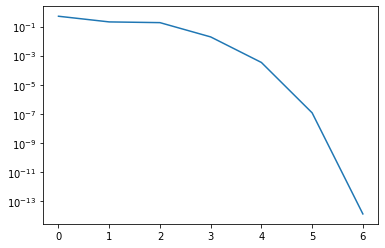
We have seen convergence in 7 iterations. Let us now reduce the matrix and continue with the next smaller matrix.
nsteps = 3

H_reduced = H[:-1, :-1] # Copy H over to preserve the original matrix

residuals = np.empty(nsteps, dtype='float64')

ident = np.eye(n-1, n-1)

for index in range(nsteps):
    shift = H_reduced[-1, -1]
    Q, R = qr(H_reduced - shift * ident)
    H_reduced = R @ Q + shift * ident
    residual = abs(H_reduced[-1, -2]) / abs(H_reduced[-1, -1])
    print(f"Residual: {residual}")
    residuals[index] = residual

plt.semilogy(residuals)
This returns
Residual: 1.0943921434074488e-05
Residual: 7.568006610141011e-11
Residual: 3.1024322351139375e-21
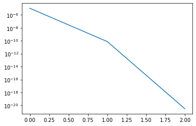
We have now observed convergence in 3 iterations. In practice, with more sophisticated shift variants and good deflation strategies the QR iteration takes typically only 2 to 3 iterations per eigenvalue, where each iteration has quadratic cost. Hence, the overall algorithm converges usually in cubic time. Even though the QR iteration is an iterative algorithm, we still speak of a method with cubic complexity, since this holds in almost all cases.
Python skills#
Below you find an implementation of the pure QR iteration.
import numpy as np

def pure_qr_iteration(A, max_iter=1000, tol=1e-10):
    """
    Computes approximate eigenvalues and eigenvectors of a real symmetric matrix A using the pure QR iteration method.

    Parameters:
    A (numpy.ndarray): The input square matrix.
    max_iter (int): Maximum number of iterations.
    tol (float): Convergence tolerance for off-diagonal elements.

    Returns:
    numpy.ndarray: Approximated eigenvalues.
    numpy.ndarray: Approximate eigenvectors.
    """
    A_k = A.copy().astype(float)  # This implementation is intended for real matrices
    n = A.shape[0]
    eigenvectors = np.eye(n)  # Accumulate eigenvectors

    for _ in range(max_iter):
        Q, R = np.linalg.qr(A_k)  # QR decomposition
        A_k = R @ Q  # Update A_k
        eigenvectors = eigenvectors @ Q  # Update eigenvectors

        # Check for convergence using the strictly lower triangular part
        off_diagonal_norm = np.linalg.norm(np.tril(A_k, k=-1))
        if off_diagonal_norm < tol:
            break

    return np.diag(A_k), eigenvectors
Let us compare the result with the build-in np.linalg.eig command:
# Define a symmetric matrix
A = np.array([[4, 1, 1], [1, 4, 1], [1, 1, 2]])

# Compute eigenvalues and eigenvectors using QR iteration
eigenvalues, eigenvectors = pure_qr_iteration(A)
eigenvectors = normalize_eigenvectors(eigenvectors)

# Display results
print("Approximated Eigenvalues:", eigenvalues)
print("Approximated Eigenvectors:\n", eigenvectors)

# Compare with NumPy's eig function
eigenvalues_np, eigenvectors_np = np.linalg.eig(A)
eigenvectors_np = normalize_eigenvectors(eigenvectors_np)
print("NumPy Eigenvalues:", eigenvalues_np)
print("NumPy Eigenvectors:\n", eigenvectors_np)
We have used here the helper function normalize_eigenvectors, which ensures eigenvectors have unit length and, for real vectors, a positive first nonzero entry.
def normalize_eigenvectors(V, tol=1e-10):
    """
    Normalizes eigenvectors such that each has unit length and, for real vectors, a positive first nonzero entry.

    Parameters:
    V (numpy.ndarray): Matrix of eigenvectors (columns are eigenvectors).
    tol (float): Tolerance below which values are considered zero.

    Returns:
    numpy.ndarray: Normalized eigenvectors.
    """
    # Normalize each column to unit length
    norms = np.linalg.norm(V, axis=0)
    norms[norms == 0] = 1  # Avoid division by zero
    V_norm = V / norms

    # Ensure the first nonzero entry of each real eigenvector is positive
    for i in range(V_norm.shape[1]):
        first_nonzero_index = np.where(V_norm[:, i] != 0)[0]  # Find nonzero indices
        if len(first_nonzero_index) > 0:
            first_nonzero = first_nonzero_index[0]  # First nonzero row index
            if np.isrealobj(V_norm) and V_norm[first_nonzero, i] < 0:
                V_norm[:, i] *= -1  # Flip sign

    # Set small values to zero
    V_norm[np.abs(V_norm) < tol] = 0.0

    return V_norm
Self-check questions#
Question
Consider two orthogonal matrices \(Q_1, Q_2 \in \mathbb{R}^{n \times n}\) and regular upper triangular matrices \(R_1, R_2 \in \mathbb{R}^{n \times n}\) such that
Then there exists a matrix \(S = \text{diag}(s_1, \ldots, s_n)\) with \(s_i \in \{-1, 1\}\) such that
Answer
By the assumptions of the question
The products and inverses of orthogonal matrices are orthogonal. Similarly, the products and inverses of regular upper triangular matrices are regular and upper triangular.
Therefore, \(S\) is upper triangular and \(S^{-1} = S^T\), implying that \(S\) is a diagonal matrix:
Again with \(S^{-1} = S^T\) we conclude \(s_i = 1/s_i\) therefore that \(s_i = 1\) or \(s_i = -1\).
Note: In conclusion, for regular matrices the QR decomposition is unique up to the choice of signs.
Question
What happens if the pure QR iteration is applied to the orthogonal matrix
Does the iteration converge? If convergence takes place, is the Schur decomposition attained in the limit and do eigenvalues appear explicitly as entries of a matrix?
You may suppose the decomposition favours positive signs on the diagonal of \(R\).
Answer
We begin by recording that the eigenvalues of \(Q\) are complex: \(\lambda_1 = i\) and \(\lambda_2 = -i\).
The pure QR iteration computes \(Q_k = Q\) and \(R_k = I\). Hence \(A_k = R_k Q_k = Q\) for every \(k\), so the iteration creates a constant sequence \((Q_k, R_k, A_k)\) and therefore converges.
In particular, \(A_k\) does not converge to an upper triangular matrix and as complex numbers do not arise in the computations, the eigenvalues do not appear explicitly as entries of a matrix.
We note that the real Schur form is attained instead, in which pairs of complex conjugate eigenvalues give rise to \(2 \times 2\) blocks on the diagonal of an almost triangular factor.
Question
What happens if the pure QR iteration is applied to the symmetric matrix
Does the iteration converge? If convergence takes place, is the Schur decomposition attained in the limit and do eigenvalues appear explicitly as entries of a matrix?
You may suppose the decomposition favours positive signs on the diagonal of \(R\).
Answer
We begin by recording that the eigenvalues of \(A\) are \(\lambda_1 = 2\) and \(\lambda_2 = 0\).
The pure QR iteration computes
From now on \(Q_k = I\) and \(R_k = A_k = A_1\). The sequence converges, and the eigenvalues are found on the diagonal of all subsequent \(A_k\).