Memory layout and NumPy#
Memory layouts#
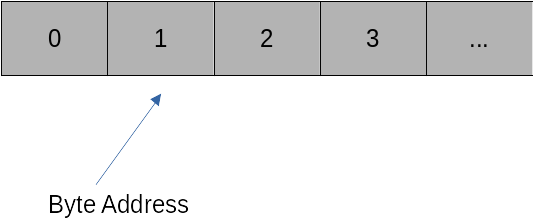
We can imagine memory as a linear collection of consecutive memory addresses, each representing one byte.
The key to efficient data representation is to arrange data so that it is spatially local in memory. This means that the data we want to work on next should be as close as possible to the data we are currently using. The reason is that memory accesses in modern computers are expensive compared to actual computations. To alleviate this problem, all modern CPUs rely on sophisticated caches that try to read data from memory ahead of time. This works only if the next pieces of data are close to the data that we are currently working on.
Standard Python list types do not guarantee this locality. List elements can be at very different memory addresses, making standard lists and other base Python types unsuitable for numerical operations. We require a buffer type that guarantees us a chunk of consecutive addresses in the system memory.
What happens if we have a matrix? Consider a \(2 \times 2\) matrix:
We have two ways of ordering this matrix in memory:
C-style ordering: This aligns the matrix row by row in memory. Hence, our memory buffer will have four elements that read:
Fortran-style ordering: This aligns the matrix column by column in memory. Our memory buffer will now have four elements that read:
Both memory layout styles are used across scientific computing, and it is important to know the assumed layout in a given numerical library. Ignoring data layouts leads to inefficiency when code has to translate on the fly between layouts, and can even cause bugs when a library makes different layout assumptions.
NumPy to the rescue#
NumPy addresses these issues by providing an array type that reserves consecutive chunks of memory and allows the user to transparently map data onto this memory, either using C-style ordering (default) or Fortran-style ordering (optional). NumPy also ensures that operations between arrays of different orderings are executed correctly (although it is best to avoid this). NumPy has long established itself as the de facto standard for array types in Python. Indeed, many other libraries have adopted the NumPy syntax and conventions to ensure their data types interoperate seamlessly with NumPy.
NumPy is one of the main reasons for Python’s success in scientific computing.
A NumPy paper was published in Nature, which is quite rare for a software library and illustrates how fundamental NumPy has become in data-driven science. Many of these operations are implemented by calling highly optimised BLAS/LAPACK routines.
BLAS and LAPACK#
BLAS (Basic Linear Algebra Subroutines) defines a set of interfaces to standard linear algebra functions. There are three BLAS variants: Level 1, 2, and 3.
BLAS Level 1 defines functions that typically require \(O(n)\) operations (\(n\) is the number of vector entries), such as vector addition, multiplication by scalars, or dot products.
BLAS Level 2 defines functions that typically require \(O(n^2)\) operations, such as matrix-vector products or triangular solves.
BLAS Level 3 defines functions that typically require \(O(n^3)\) operations, of which the most important one is the matrix-matrix product.
A reference BLAS implementation exists from http://www.netlib.org. However, this should never be used in practice. The key to fast BLAS operations is implementations that optimally use the CPU cache architecture to minimise data transfer delays. Several BLAS libraries exist that are optimised for modern CPUs and not only exploit caching but also SIMD acceleration and multi-core processing. Examples of such libraries are Intel MKL, OpenBLAS, or BLIS.
LAPACK is a library of advanced linear algebra functions such as linear system solves, eigenvalue problems, singular value problems, and least-squares problems, built on top of BLAS. LAPACK routines are designed to use Level-3 BLAS matrix-matrix operations whenever possible. The reason is memory efficiency. For matrix-matrix products, the arithmetic cost scales like \(O(n^3)\) whereas the data volume scales like \(O(n^2)\). Hence, for larger problems, we have far more operations than memory accesses, which is desirable because memory accesses are slow.
NumPy links against available BLAS and LAPACK libraries to ensure efficient implementations of linear algebra operations. Which backend is used depends on how NumPy was installed; common choices include OpenBLAS and Intel MKL.
Python skills#
We already know that NumPy is a fundamental library for scientific computing in Python. Here’s a quick introduction to its basic features and functionality. To use NumPy, import it as follows:
import numpy as np
Creating Arrays#
The basic data type in NumPy is the array. Here are some examples of how to create arrays:
# A double-precision array with three entries
a = np.array([3.5, 4, 18.1], dtype='float64')

# Random array with 10 components
a_random = np.random.rand(10)

# A 10x10 matrix of ones, stored as double precision
a_ones = np.ones((10, 10), dtype='float64')

# A complex 3D tensor with all entries set to zero
a_zeros = np.zeros((10, 10, 10), dtype='complex128')

# An uninitialized byte array that can store 50 bytes
a_empty = np.empty(50, dtype='byte')

# The first 50 integers, starting at 0
a_range = np.arange(50)
Accessing Array Properties#
You can easily access the shape of an array:
print(a_range.shape)  # (50,)
print(a_zeros.shape)  # (10, 10, 10)
Accessing Elements#
Accessing elements of arrays is straightforward:
# Access the first element
a_random[0]

# Access the first two elements
a_random[:2]

# Access the last two elements
a_random[-2:]

# Access a submatrix (third to fifth column in the first three rows)
a_ones[:3, 2:5]

# Access an element in a multidimensional array
a_zeros[3, 2, 1]
Modifying Arrays#
You can also modify elements of arrays:
# Set a specific element
a_ones[3, 3] = 10

# Set a column to a range of values
a_ones[:, 4] = np.arange(10)

# Set an entire row to a specific value
a_ones[8] = 10
Plotting with NumPy and Matplotlib#
Together with Matplotlib, you can easily plot data:
from matplotlib import pyplot as plt

x = np.linspace(-10, 10, 10000)
y = np.exp(-x**2)

plt.plot(x, y)
plt.xlabel('x')
plt.ylabel('exp(-x^2)')
plt.show()
Matrix Operations#
Matrix and vector operations in NumPy include:
# Generate random matrices
A = np.random.randn(100, 100)
B = np.random.randn(100, 100)

# Matrix/matrix product
C = A @ B

# Componentwise product
C_elementwise = A * B
Solving Linear Systems#
NumPy can solve linear systems of equations:
A = np.random.rand(1000, 1000)
b = np.random.rand(1000)

# Solve Ax = b
x = np.linalg.solve(A, b)

# Compute the relative residual
residual = np.linalg.norm(b - A @ x) / (np.linalg.norm(A) * np.linalg.norm(x) + np.linalg.norm(b))
print(residual)
This computation typically gives a relative residual close to machine precision.
Further Resources#
For a more comprehensive introduction, refer to the NumPy user guide.