Polynomial Interpolation

Polynomial Interpolation#

The set of real polynomials of degree less than or equal to $n$ is denoted by $\mathcal{P}_n$. We consider the following task:

Given $n+1$ distinct points $x_0,x_1,\dots,x_n$, and $n+1$ values $y_0,y_1,\dots,y_n$, find a polynomial $p_n \in \mathcal{P}_n$ such that

\[ p(x_j)=y_j \qquad \forall j \in \{ 0, \ldots, n \}. \]

In this section, we will answer the following questions:

Does a polynomial $p_n$ with $p_n(x_j)=y_j$ always exist, and if yes, is it unique?
How can we construct such a polynomial in practice?
If the values $y_j$ are samples of a function, do we observe convergence to the function as $n\rightarrow\infty$?

To begin with, we consider the special case

\[ y_j = \delta_{ij}, \]

meaning that $y_i = 1$ and $y_j = 0$ for $i \neq j$. It has the solution

\[ L_j(x)= \prod_{i=0,i \neq j}^n \frac{(x-x_i)}{(x_j-x_i)}. \]

because $\text{deg}(L_j)=n$ and $L_j$ interpolates $y_j = \delta_{ij}$ at $x_j$. The functions $L_k$ are called Lagrange basis polynomials.

The solution to the original interpolation problem is now constructed as

\[ p_n(x)= \sum_{j=0}^n y_j L_j(x). \]

We refer to $p$, when written in this form, as the Lagrange interpolation polynomial. We still need to prove uniqueness.

Theorem 4 (Existence and uniqueness of interpolating polynomial)

Given $\{ (x_i,y_i) \}_{i=0}^n$ with $x_i < x_{i+1}$, there exists a unique $p_n \in \mathcal{P}_n$ such that $p_n(x_i) = y_i$ for all $i = 0, \ldots, n$.

Proof. Let $q_n(x)$ be another polynomial of degree at most $n$ that satisfies $q_n(x_j)=y_j$. Let $w_n:=p_n-q_n$. We then have $w(x_j)=0$, $j=0,\dots,n$. Hence, $w_n$ is a polynomial of maximum degree $n$ with $n+1$ distinct zeros. However, since a nontrivial polynomial of degree $n$ can have at most $n$ zeros, it follows that $w\equiv 0$, showing that $p_n$ is the unique interpolation polynomial.

We denote the error polynomial by

\[ \omega_{n+1}(x) := \prod_{j = 0}^n (x - x_j). \]

Theorem 5 (Interpolation error bound)

Suppose $f \in C^{n+1}[a,b]$ and $a \le x_0 < \ldots < x_n \le b$. Let $p \in \mathcal{P}_n$ such that $p(x_i) = f(x_i)$ for $i \in \{ 0, \dots, n\}$. Then for every $x \in [a,b]$ there is a $\xi \in [a,b]$, depending on $x$, such that

\[ f(x) - p(x) = \frac{\omega_{n+1}(x) f^{(n+1)}(\xi)}{(n+1)!}. \]

The proof is given in the optional materials section. One disadvantage of the above interpolation error bound is that the result only applies to $f \in C^{n+1}[a,b]$. The celebrated Weierstrass approximation theorem shows that control on higher-order derivatives is not necessary for the approximation by polynomials.

Fact: Weierstrass approximation theorem

Given $f \in C[a,b]$ and $\epsilon > 0$, there exists an $n \in \mathbb{N}$ and $p \in \mathcal{P}_n$ such that $\| f - p \|_\infty < \epsilon$.

Here $\| g \|_\infty = \max_{x \in [a,b]} |g(x)|$ denotes the $\infty$-norm on $C[a,b]$.

The $p$ of the Weierstrass approximation theorem has to be selected with much care, and an unrefined interpolation method will generally not provide polynomials which approximate arbitrarily well. This is mainly due to the Runge phenomenon.

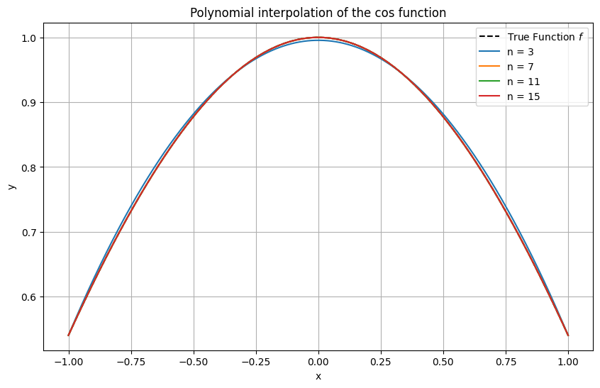
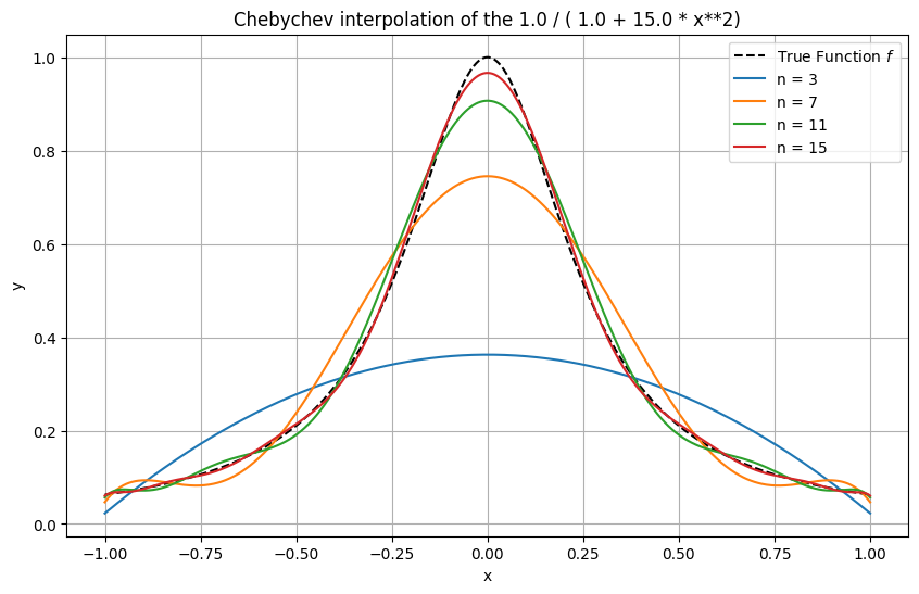
Example 4 (Interpolation with uniformly distributed nodes)

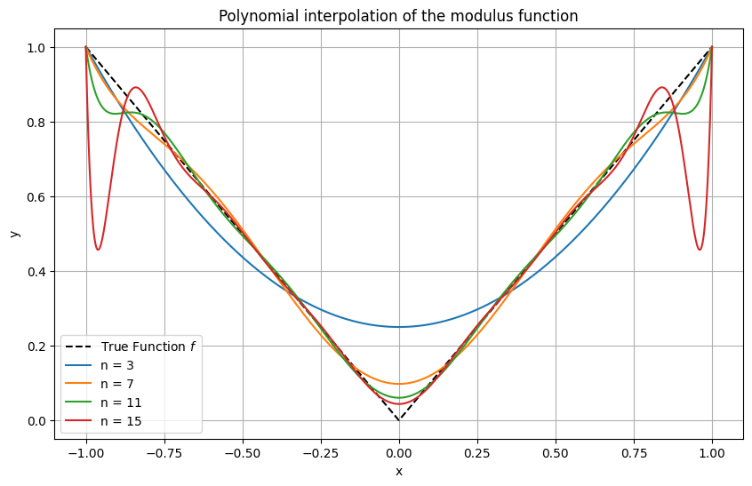
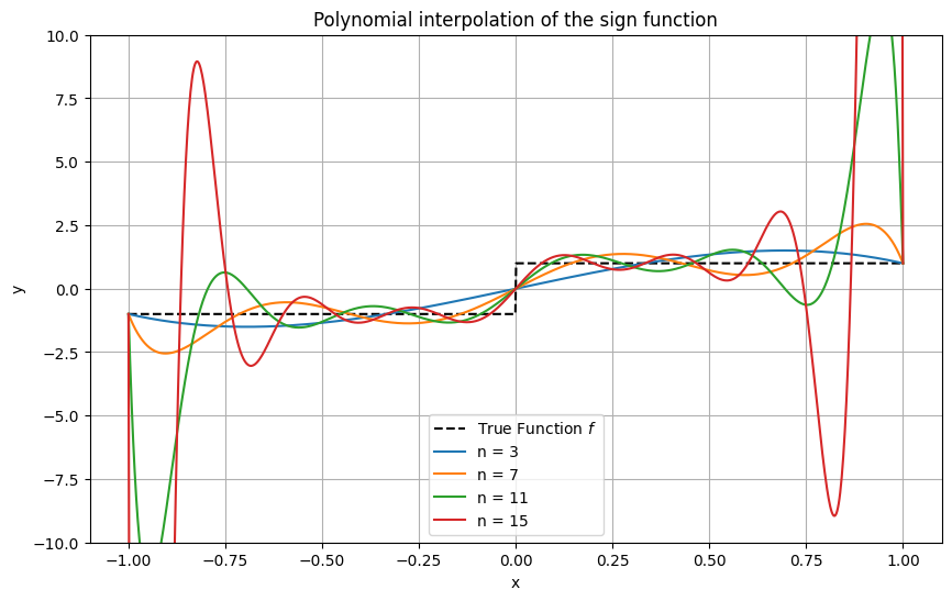
Unless very smooth functions such as $\cos$ are interpolated (recall that $\| \cos^{(n)} \|_\infty = 1$ for all $n$th derivatives $\cos^{(n)}$, $n \in \mathbb{N}$), one observes that interpolating polynomials of high-order exhibit strong oscillations near the interval ends. This behaviour is known as the Runge phenomenon.

Click through the tabs to see:

An example with infinitely many uniformly bounded derivatives.
An example with infinitely many derivatives.
An example with a continuous function.
An example with a discontinuous function.

cos(x)

cos

1 / (1 + 15 x^2)

$fraction$

abs(x)

cos

sign(x)

cos

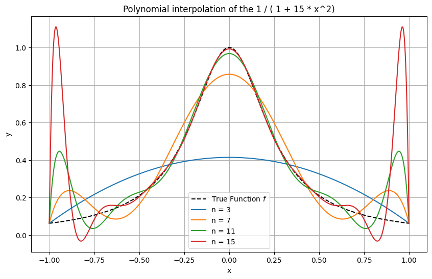
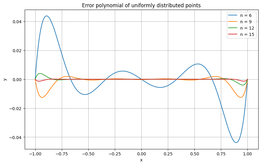
To understand the Runge phenomenon, it is instructive to examine the error term

\[ \frac{1}{(n+1!)} \, \omega_{n+1}(x) \, f^{(n+1)}(\xi) = E(x), \qquad x \in (x_0, x_n) \]

more carefully for $C^\infty$ functions such as the $x \mapsto \frac{1}{1 + 15 x^2}$ of the previous example. It consists of three parts:

the scaling factor $(n+1!)^{-1}$;
the error polynomial $\omega_{n+1}(x)$, which measures how well the nodes are chosen;
the derivative $f^{(n+1)}(\xi)$, which measures how difficult it is to approximate $f$.

The following plot illustrates how the error polynomial attains its largest values near the domain boundaries.

error_polynomial

Note that the error polynomial’s $\infty$-norm decreases as $n \to \infty$; however, it is not fast enough to counter the often observed increase in the magnitude of $f^{(n+1)}(\xi)$ as $n \to \infty$.

Can nodes be distributed non-uniformly to better reduce the magnitude of $\omega$ throughout the interpolation domain? In other words, is there a distribution of nodes $\{\tilde{x}_0, \ldots, \tilde{x}_m \}$ which has the smallest error polynomial $\tilde{\omega}_{n+1}$?

There is indeed such a choice of nodes: these are the roots of Chebychev polynomials. For $n \in \mathbb{N}$ they are defined as

\[ \tilde{x}_i = \cos \Bigl( \frac{2 i + 1}{2 n} \pi \Bigr), \qquad i \in \{ 0, \ldots, n\}. \]

(Note: Some texts define $i$ to start from $1$ in the definition of Chebyshev nodes and adjust $n$ accordingly. This is only a notational difference.)

Theorem 6

Consider $n+1$ arbitrary, pairwise distinct nodes $x_0, x_1, \ldots, x_n$ in $[-1,1]$ with error polynomial $\omega_{n+1}$. Then

\[ \| \tilde{\omega}_{n+1} \|_\infty \le \| \omega_{n+1} \|_\infty, \]

$\tilde{\omega}_{n+1}$ is the error polynomial of the Chebyshev nodes.

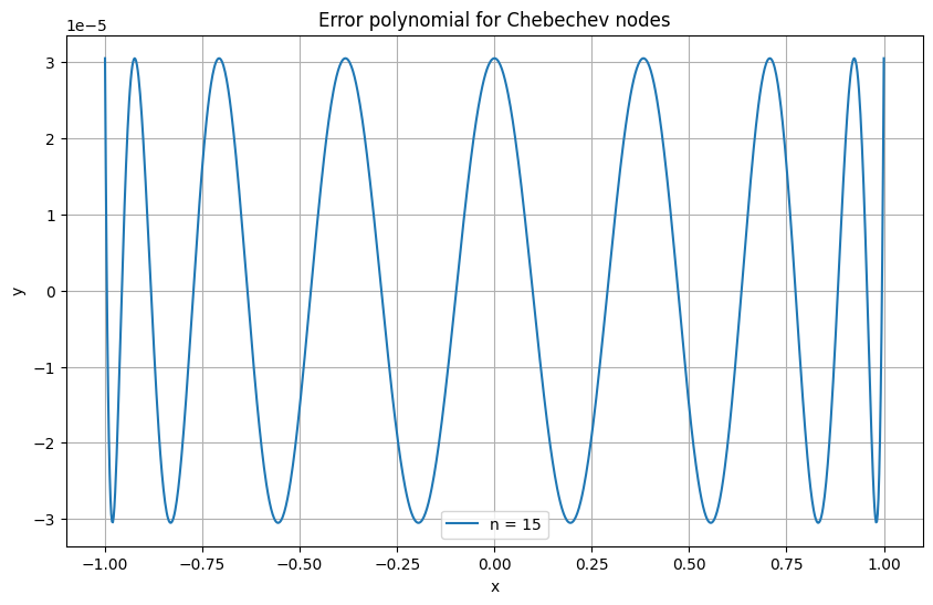
The proof is given in the optional materials section. Important for us is that Chebychev nodes address the issue of Runge’s phenomenon successfully, as illustrated in the following example.

The trick here is that Chebychev nodes have a finer spacing near the interval boundary, preventing the error polynomial’s strong oscillations.

error_polynomial

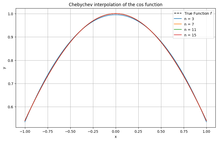
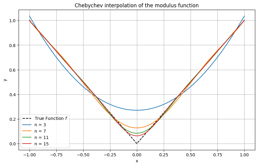
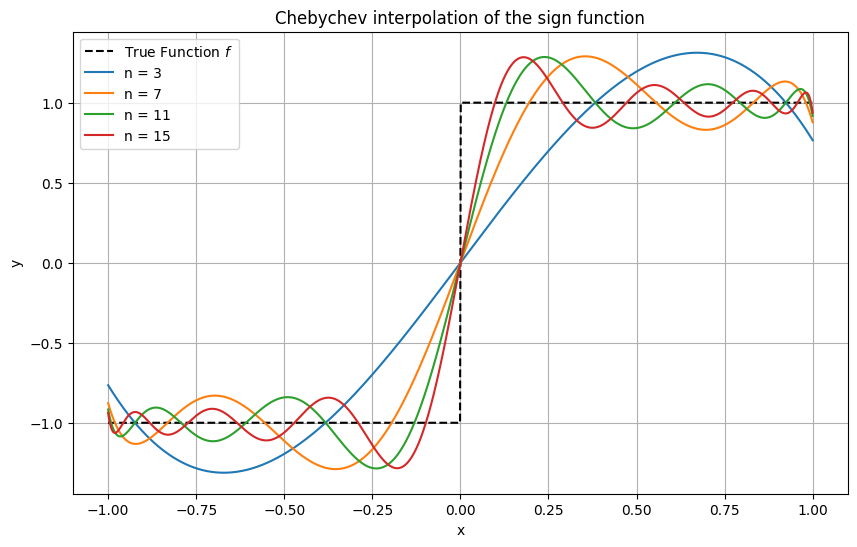
Example 5 (Interpolation with Chebychev nodes)

Here, the same functions as above are interpolated again, this time using Chebychev nodes. The difference is striking, with a fairly good approximation even in the discontinuous example of the sign function.

cos(x)

cos

1 / (1 + 15 x^2)

$fraction$

abs(x)

abs

sign(x)

sign

Python skills#

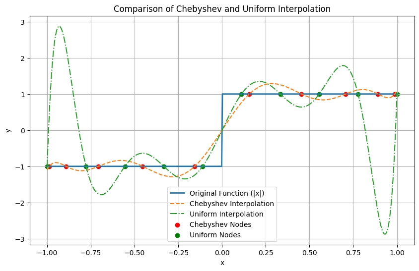
The following code implements Lagrange interpolation and compares Chebychev and uniform interpolation of the sign function in a single plot.

import numpy as np
import matplotlib.pyplot as plt


def chebyshev_nodes(n):
    """Generate Chebyshev nodes."""
    return np.cos((2 * np.arange(1, n + 1) - 1) * np.pi / (2 * n))


def uniform_nodes(n):
    """Generate uniform nodes."""
    return np.linspace(-1, 1, n)


def lagrange_interpolation(nodes, f, x_eval):
    """Perform Lagrange interpolation using given nodes."""

    def lagrange_basis(x, k):
        term = 1
        for j in range(len(nodes)):
            if j != k:
                term *= (x - nodes[j]) / (nodes[k] - nodes[j])
        return term

    y_eval = np.zeros_like(x_eval)
    for k in range(len(nodes)):
        y_eval += f(nodes[k]) * lagrange_basis(x_eval, k)

    return y_eval


# Non-smooth function to interpolate
f = lambda x: np.sign(x)

# Number of nodes
n = 10

# Evaluation points
x_eval = np.linspace(-1, 1, 500)

# Perform Lagrange interpolation with Chebyshev and Uniform nodes
y_interp_chebyshev = lagrange_interpolation(chebyshev_nodes(n), f, x_eval)
y_interp_uniform = lagrange_interpolation(uniform_nodes(n), f, x_eval)

# Plot
plt.figure(figsize=(10, 6))
plt.plot(x_eval, f(x_eval), label='Original Function (|x|)', linewidth=2)
plt.plot(x_eval, y_interp_chebyshev, '--', label='Chebyshev Interpolation')
plt.plot(x_eval, y_interp_uniform, '-.', label='Uniform Interpolation')
plt.scatter(chebyshev_nodes(n), f(chebyshev_nodes(n)), color='red', label='Chebyshev Nodes')
plt.scatter(uniform_nodes(n), f(uniform_nodes(n)), color='green', label='Uniform Nodes')
plt.xlabel('x')
plt.ylabel('y')
plt.title('Comparison of Chebyshev and Uniform Interpolation')
plt.legend()
plt.grid(True)
plt.show()

Notice how the spacing of Chebychev nodes is tighter near the interval ends:

cheb_uniform

Lagrange interpolation and related methods are built into Scipy, see this link.

Self-check questions#

Question

Given the nodes $\{x_0, \ldots, x_n\}$, show that the linearity of the mapping

\[ \mathbb{R}^{n+1} \to \mathcal{P}_n, (y_0, y_1, \ldots, y_n)^T \mapsto p, \]

where $p \in \mathcal{P}_n$ is the polynomial interpolating the values $y_i$.

Question

Consider the following set of data points:

$(x_0, y_0) = (1, 1)$
$(x_1, y_1) = (2, 3)$
$(x_2, y_2) = (3, 2)$

Calculate the Lagrange interpolating polynomial that passes through these points.

Question

Suppose that the interpolation nodes are arranged symmetrically around the origin: for each node $x_j$, the node $-x_j$ also exists in the set of nodes.

Prove that the Lagrange interpolant $p$ of an odd function is odd.

Polynomial Interpolation

Contents

Polynomial Interpolation#

Python skills#

Self-check questions#

Optional material#