Least Squares Problems

Least squares problems occur in optimisation, data fitting and other fields of the mathematical sciences.

Consider a matrix \(A \in \mathbb{R}^{m \times n}\) and a vector \(b \in \mathbb{R}^m\). The central idea of the least squares problem is to find a vector \(\hat{x} \in \mathbb{R}^n\) that minimises the Euclidean norm (or \(2\)-norm) of the residual vector \(Ax - b\). This problem is formulated as

\[ \hat{x} \in \text{arg}\min_{x \in \mathbb{R}^n} \|Ax - b\|_2. \]

Here \(\text{arg}\min_{x \in \mathbb{R}^n} \|Ax - b\|_2\) is the set of all \(x\) which minimise \(\|Ax - b\|_2\). If the minimiser is unique, we also write (with a slight abuse of notation)

\[ \hat{x} = \text{arg}\min_{x \in \mathbb{R}^n} \|Ax - b\|_2. \]

Thus, in the least squares sense, the optimisation problem generalises the concept of the solution to a system of linear equations: if \(A\) is invertible, then \(A \hat{x} = b\). If \(A\) is overdetermined, then \(\hat{x}\) aims to minimise the amount by which \(A \hat{x}\) fails to achieve equality with \(b\).

The normal equation

The identity

\[ A^TA\hat{x} = A^Tb. \]

is called the normal equation of the least-squares problem.

Theorem 3 (Normal equation of least-squares approximations)

Let \(A \in \mathbb{R}^{m \times n}\), \(b \in \mathbb{R}^m\). Then

\[ \hat{x} \in \text{arg}\min_{x \in \mathbb{R}^n} \|Ax - b\|_2. \]

if and only if \(\hat{x}\) satisfies the normal equation.

Proof. The vector \(\hat{x}\) minimises the least-squares problem if and only if for all \(\epsilon\in\mathbb{R}^n\):

\[\begin{split} \begin{aligned} \|A\hat{x} -b \|_2^2 & \leq \|A(\hat{x} + \epsilon) - b\|_2^2 = \left[A(\hat{x} + \epsilon) - b\right]^T\left[A(\hat{x} + \epsilon) - b\right]\\ &= \|A\hat{x} -b \|_2^2+2 \epsilon^T(A^TA\hat{x} - A^Tb) + \epsilon^TA^TA\epsilon \end{aligned} \end{split}\]

Step 1: Suppose that \(\hat{x}\) does not satisfy the normal equation. Then \(\| A^TA\hat{x} - A^Tb \|_2 > 0\). Suppose that \(\hat{x}\) minimises the least-squares problem. With \(\epsilon := \delta (A^TA\hat{x} - A^Tb)\), \(\delta \in \mathbb{R}\), the above implies

\[ 0 \leq 2 \delta \, \| A^TA\hat{x} - A^Tb \|_2^2 + \delta^2 \, \| A (A^TA\hat{x} - A^Tb) \|_2^2 =: \Phi(\delta) \qquad \forall \delta \in \mathbb{R}. \]

This is a contradiction because \(\Phi(\delta) < 0\) for small negative \(\delta\).

Step 2: Suppose that \(\hat{x}\) satisfies the normal equation. Then, by the above,

\[ \|A(\hat{x} + \epsilon) - b\|_2^2 = \|A\hat{x} -b \|_2^2 + \epsilon^TA^TA\epsilon \geq \|A\hat{x} -b \|_2^2. \]

Properties of the normal equation

We assume in this section that \(m \ge n\) and that \(A\) has a full rank. Let \(A = U\Sigma V^T \in \mathbb{R}^{m \times n}\) be the SVD of \(A\). To generalise the relative condition number of a square matrix, we define the relative condition number for a rectangular \((m \times n)\)-matrix as

\[ \kappa_{rel}(A):=\sigma_1/\sigma_n. \]

We also have

\[ A^TA = V\Sigma^T\Sigma V^T \in \mathbb{R}^{n \times n}, \]

guaranteeing the non-singularity of \(A^T A\) and, therefore, the existence of a unique minimiser of the least-squares problem.

Furthermore,

\[ \kappa_{rel}(A^TA) = \sigma_1^2 / \sigma_n^2 = \kappa_{rel}(A)^2. \]

It follows that the linear system in the normal equation has a squared condition number compared to the original matrix \(A\).

Subsequently, we will explore orthogonalisation methods to circumvent this condition number squaring, offering a more stable approach to solving the least-squares problem.

Solving least-squares problems with the QR decomposition

We assume in this section that \(m \ge n\) and that \(A\) has a full rank. The full \(QR\) decomposition of \(A\) can be expressed as follows:

\[\begin{split} A = \begin{bmatrix} Q_1 & Q_2 \end{bmatrix}\begin{bmatrix} R \\ 0 \end{bmatrix}, \end{split}\]

where \(Q_1\) and \(Q_2\) are orthogonal matrices, and \(R\) is an upper triangular matrix. Substituting this decomposition into the least-squares problem, we get:

\[\begin{split} \|Ax - b\|_2 = \left\|\begin{bmatrix} Q_1 & Q_2 \end{bmatrix}\begin{bmatrix} R \\ 0 \end{bmatrix}x - b\right\|_2 = \left\|\begin{bmatrix} R \\ 0 \end{bmatrix}x - \begin{bmatrix} Q_1^Tb \\ Q_2^Tb \end{bmatrix}\right\|_2 \end{split}\]

Here, we observe that the choice of \(x\) influences only the first block-row. In the second block row, \(x\) is multiplied by zero, meaning no choice of \(x\) will reduce the contribution from this part. Therefore, the minimiser \(\hat{x}\) of the least squares problem is found by solving:

\[ R \hat{x} = Q_1^Tb. \]

Returning to the question of the \(2\)-norm condition number:

\[ \kappa_{rel}(R) = \kappa_{rel}(Q^T A) = \| Q^T A \|_2 \, \| (Q^T A)^{-1} \|_2 \leq \| Q^T \|_2 \, \| A \|_2 \, \| A^{-1} \|_2 \, \| Q \|_2 = \kappa_{rel}(A), \]

where we use the submultiplicativity of the matrix \(2\)-norm and that \(\| Q \|_2 = 1\) and \(Q^T = Q^{-1}\).

Consequently, the \(QR\) decomposition approach effectively circumvents the condition number squaring issue associated with the normal equation method.

Solving least-squares problems with the SVD

The SVD can also be used to solve least-squares problems. In this section, we assume that \(m \ge n\) but not that \(A\) has a full rank. The full SVD of \(A\) is

\[\begin{split} A = U\Sigma V^T = \begin{bmatrix} U_1 & U_2 \end{bmatrix} \begin{bmatrix} \hat{\Sigma} & 0 \\ 0 & 0 \end{bmatrix} \begin{bmatrix} V_1 & V_2 \end{bmatrix}^T \end{split}\]

with \(\hat{\Sigma}\) as in the previous chapter. Substitute into the least-squares problem to obtain

\[ \|Ax-b\|_2 = \|U\Sigma V^Tx - b\|_2. \]

Let \([y_1, y_2]^T = [V_1^T x, V_2^T x]^T\) and factorise out \(U\) to obtain

\[\begin{split} \|Ax - b\|_2 = \left\|\begin{bmatrix} \hat{\Sigma} & 0 \\ 0 & 0 \end{bmatrix} \begin{bmatrix} y_1\\ y_2 \end{bmatrix} - \begin{bmatrix}U_1^Tb\\ U_2^Tb\end{bmatrix}\right\|_2. \end{split}\]

The second block row as well as the choice of \(y_2\) do not affect the least-squares norm and, hence, \(y_1 = \hat{\Sigma}^{-1} U_1^Tb\) and therefore

\[\begin{split} \hat{x}= \begin{bmatrix} V_1 & V_2 \end{bmatrix} \begin{bmatrix} \hat{\Sigma}^{-1} & 0 \\ 0 & 0 \end{bmatrix} \begin{bmatrix} U_1 & U_2 \end{bmatrix}^T b \end{split}\]

is a (possibly non-unique) minimiser of the least-squares problem. This leads to the important concept of a pseudo-inverse of a matrix.

Definition 1 (Pseudo-inverse of a matrix)

Let \(U \Sigma V^T\) be an SVD of \(A \in \mathbb{R}^{m \times n}\) and \(m \geq n\). Then the pseudo-inverse of \(A\) is

\[\begin{split} A^{\dagger} := V \begin{bmatrix} \hat{\Sigma}^{-1} & 0 \\ 0 & 0 \end{bmatrix} U^T, \end{split}\]

where \(\hat{\Sigma} \in \mathbb{R}^{r \times r}\) and \(r = \text{rank}(A)\).

The pseudo-inverse of \(A\) is a generalisation of the inverse of \(A\). In the same way that \(A^{-1}b\) solves the linear system \(Ax=b\) for a square matrix \(A\), the pseudo-inverse \(A^{\dagger}\) applied to \(b\) solves the least-squares minimisation problem \(\|Ax-b\|_2\) for rectangular \(A\).

Python skills

Solving a least-squares problem with QR decomposition

The following example shows how to use Numpy’s QR decomposition to find the least-squares approximation

import numpy as np
from scipy.linalg import solve_triangular

# Define matrix A and vector b
A = np.array([[1, 2], [3, 4], [5, 6]])
b = np.array([7, 8, 9])

# Perform QR decomposition
Q, R = np.linalg.qr(A)

# Compute Q^T * b
Q_T_b = np.dot(Q.T, b)

# Solve Rx = Q^Tb for x
x = solve_triangular(R[:A.shape[1], :], Q_T_b[:A.shape[1]])

print("Solution x:", x)

Solving a least-squares problem with SVD

Here is a problem that is solved with the SVD.

import numpy as np

# Step 1: Define A and b
A = np.random.rand(5, 3)  # A random 5x3 matrix
b = np.random.rand(5)  # A random vector of length 5

# Step 2: Perform SVD
U, sigma, VT = np.linalg.svd(A)

# Step 3: Compute the pseudo-inverse
Sigma_inv = np.hstack((np.diag(1 / sigma), np.zeros((3, 2))))
A_pseudo_inverse = VT.T @ Sigma_inv @ U.T

# Step 4: Solve for x
x = A_pseudo_inverse @ b

print("Solution x:", x)

Self-check questions

Question

Let’s consider three points: \((1, 2)\), \((2, 3)\), and \((3, 5)\). Find the best-fitting line \(y = m x + c\) in the least-squares sense:

\[ (\hat{c}, \hat{m}) = \text{arg}\min_{(c,m) \in \mathbb{R}^2} | 2 - (m \, 1 + c) |^2 + | 3 - (m \, 2 + c) |^2 + | 5 - (m \, 3 + c) |^2. \]

Answer

The minimisation problem can be equivalently formulated as

\[\begin{split} \text{arg}\min_{(c,m) \in \mathbb{R}^2} \left\| \begin{bmatrix} 1 & 1\\ 1 & 2\\ 1 & 3 \end{bmatrix} \begin{bmatrix} c\\ m \end{bmatrix} - \begin{bmatrix} 2\\ 3\\ 5 \end{bmatrix} \right\|^2. \end{split}\]

We learned three methods to proceed: solve the normal equation, the QR reformulation or the SVD reformulation. The two latter choices are preferable for bigger problems solved with a computer. However, for hand calculations of small problems, solving the original normal equation is often the most convenient approach.

We have

\[\begin{split} \mathbf{A}^T\mathbf{A} = \begin{bmatrix} 1 & 1 & 1\\ 1 & 2 & 3 \end{bmatrix} \begin{bmatrix} 1 & 1 \\ 1 & 2 \\ 1 & 3 \end{bmatrix} = \begin{bmatrix} 3 & 6 \\ 6 & 14 \end{bmatrix} \end{split}\]

and

\[\begin{split} \mathbf{A}^T\mathbf{b} = \begin{bmatrix} 1 & 1 & 1\\ 1 & 2 & 3 \end{bmatrix} \begin{bmatrix} 2 \\ 3 \\ 5 \end{bmatrix} = \begin{bmatrix} 10\\ 23 \end{bmatrix}. \end{split}\]

Thus, the minimiser solves

\[\begin{split} \begin{bmatrix} 3 & 6 \\ 6 & 14 \end{bmatrix} \begin{bmatrix} c \\ m \end{bmatrix} = \begin{bmatrix} 10\\ 23 \end{bmatrix}, \end{split}\]

giving \((\hat{c}, \hat{m}) = (1/3, 3/2)\).

Remark One can plot an illustration of the calculation with Python.

import matplotlib.pyplot as plt
import numpy as np

# Given points
x_points = np.array([1, 2, 3])
y_points = np.array([2, 3, 5])

# Given least-squares solution
c = 1.0/3.0
m = 3.0/2.0

# Line of best fit
x_line = np.linspace(0, 4, 100)
y_line = m * x_line + c

# Plotting
plt.figure(figsize=(8, 6))
plt.plot(x_line, y_line, label=f'Best Fit Line: y = {m:.2f}x + {c:.2f}', color='red')
plt.scatter(x_points, y_points, label='Data Points', color='blue')
plt.xlabel('x')
plt.ylabel('y')
plt.title('Least Squares Line Fit')
plt.legend()
plt.grid(True)
plt.show()

Question

Let \(x=(0,0.25,0.5,0.75,1)\).

1. Find a least-squares quadratic approximation to \(\{(x_i,\exp(x_i))\}\).

2. Find a least-squares quadratic approximation to \(\{(x_i,\cos(x_i))\}\).

Answer

1. The quadratic approximation is of the form \(p_2(x) = a \, x^2 + b \, x + c\). The minimisation problem can be equivalently formulated as

   \[\begin{split} \text{arg}\min_{(a,b,c) \in \mathbb{R}^3} \left\| \begin{bmatrix} x_1^2 & x_1 & 1\\ x_2^2 & x_2 & 1\\ x_3^2 & x_3 & 1\\ x_4^2 & x_4 & 1\\ x_5^2 & x_5 & 1\end{bmatrix} \begin{bmatrix} a\\ b\\ c \end{bmatrix} - \begin{bmatrix} \exp(x_1)\\ \exp(x_2)\\ \exp(x_3)\\ \exp(x_4)\\ \exp(x_5) \end{bmatrix} \right\|^2. \end{split}\]

   The normal equations in matrix form are:

   \[\begin{split} \begin{bmatrix} \sum_i x_i^4 & \sum_i x_i^3 & \sum_i x_i^2 \\ \sum_i x_i^3 & \sum_i x_i^2 & \sum_i x_i \\ \sum_i x_i^2 & \sum_i x_i & n \end{bmatrix} \begin{bmatrix} a \\ b \\ c \end{bmatrix} = \begin{bmatrix} \sum_i (x_i^2 y_i) \\ \sum_i (x_i y_i) \\ \sum_i y_i \end{bmatrix} \end{split}\]

   where \(y_i = \exp(x_i)\) and \(n\) is the number of data points. Therefore, the least-squares quadratic approximation is given by:

   \[ p_2(t)=1.005+0.8643t+0.8435t^2. \]

2. Analogously, the approximation is \(p_2(t)=1.001-0.03389t-0.4288t^2\).

Question

For many applications, one must obtain polynomial least-squares approximations at the same nodes \(\{ x_i \}\) for many different sets of data \(\{y_i\}\). What is the best way to do this? Only try to answer this after having worked out the two previous questions.

Answer

The matrix \(A\) of the normal equation \(A^TA\hat{x} = A^Tb\) depends on \(\{ x_i \}\), but not \(\{y_i\}\). Compute the QR or singular value decomposition of \(A\) once, and apply it for each of the different \(\{y_i\}\).

Question

Let \(A\in\mathbb{R}^{m\times n}\) with \(m\geq n\) and \(\text{rank}(A)=n\) and \(b\in\mathbb{R}^m\). How should one approach the following least-squares problem with the SVD? Find \(\hat{x}\in\mathbb{R}^n\), such that

\[ \|A\hat{x}-b\|_2 = \min_{x\in\mathbb{R}^n}\|Ax-b\|_2. \]

Answer

The SVD of \(A\) is given as \(A=U\Sigma V^T\), where \(U\in\mathbb{R}^{m\times m}\) and \(V\in\mathbb{R}^{n\times n}\) are orthogonal matrices and \(\Sigma \in\mathbb{R}^{m\times n}\) is a diagonal matrix with the nonzero singular values \(\sigma_1\geq\sigma_2\geq\dots\geq\sigma_n >0\) in decreasing order on the diagonal of the matrix, using that \(A\) has full rank.

Substituting into the least-squares problem, we have

\[ \|Ax-b\|_2 = \|U\Sigma V^Tx - b\|_2 = \|\Sigma y - \hat{b}\|_2 \]

for \(y=V^Tx\) and \(\hat{b} = U^Tb\). We find \(y_j\) as \(y_j = \hat{b}_j/\sigma_j\) by minimising the above expression. This is equivalent to \(x = A^{\dagger} b\).

Question

We now consider the modified least-squares problem

\[ \min_{x\in\mathbb{R}^n} \|Ax-b\|_2^2+\|L x\|_2^2 \]

with \(L\in\mathbb{R}^{n\times n}\) nonsingular. Show that the solution of this least-squares problem is identical to the solution of

\[ (A^TA+L^TL)x = A^Tb. \]

Answer

The vector \(\hat{x}\) minimises the least-squares problem if and only if for all \(\epsilon\in\mathbb{R}^n\):

\[\begin{split} \begin{aligned} \|A\hat{x} -b \|_2^2 + \| L \hat{x}\|_2^2 & \leq \|A(\hat{x} + \epsilon) - b\|_2^2 + \| L (\hat{x} + \epsilon) \|_2^2\\ & = \left[A(\hat{x} + \epsilon) - b\right]^T\left[A(\hat{x} + \epsilon) - b\right] + [L (\hat{x} + \epsilon)]^T [L (\hat{x} + \epsilon)]\\ &= \|A\hat{x} -b \|_2^2+2 \epsilon^T(A^TA\hat{x} - A^Tb) + \epsilon^TA^TA\epsilon + \|L\hat{x} \|_2^2+2 \epsilon^T(L^TL\hat{x}) + \epsilon^TL^T L \epsilon\\ &= \|A\hat{x} -b \|_2^2 + \|L\hat{x} \|_2^2 + 2 \epsilon^T((A^TA + L^TL) \hat{x} - A^Tb) + \epsilon^T(A^TA + L^T L) \epsilon \end{aligned} \end{split}\]

Step 1: Suppose that \(\hat{x}\) does not satisfy the generalised normal equation \((A^TA+L^TL)x = A^Tb.\). Then \(\| (A^TA + L^TL) \hat{x} - A^Tb \|_2 > 0\). Suppose that \(\hat{x}\) minimises the least-squares problem. With \(\epsilon := \delta ((A^TA + L^TL) \hat{x} - A^Tb)\), \(\delta \in \mathbb{R}\), the above implies

\[ 0 \leq 2 \delta \, \| (A^TA + L^TL) \hat{x} - A^Tb \|_2^2 + \delta^2 \, \| (A + L) ((A^TA + L^TL) \hat{x} - A^Tb) \|_2^2 =: \Phi(\delta) \qquad \forall \delta \in \mathbb{R}. \]

This is a contradiction because \(\Phi(\delta) < 0\) for small negative \(\delta\).

Step 2: Suppose that \(\hat{x}\) satisfies the generalised normal equation. Then, by the above,

\[ \|\|A(\hat{x} + \epsilon) - b\|_2^2 + \| L (\hat{x} + \epsilon) \|_2^2 = \|A\hat{x} -b \|_2^2 + \|L\hat{x} \|_2^2 + \epsilon^T(A^TA + L^T L) \epsilon \geq \|A\hat{x} -b \|_2^2 + \|L\hat{x} \|_2^2, \]

ensuring that \(\hat{x}\) is a minimiser.

Question

Let \(A = QR\) be the QR decomposition of a matrix \(A\in\mathbb{R}^{m\times n}\) with \(R\in\mathbb{R}^{n\times n}\). Show that the singular values of \(A\) are identical to those of \(R\).

Answer

We use the full QR decomposition; that is, let

\[\begin{split} A = \begin{bmatrix}Q & Q^{\bot}\end{bmatrix}\begin{bmatrix}R\\ 0\end{bmatrix}. \end{split}\]

Let \(R = U\Sigma V^T\) be the SVD of \(R\). Plugging into the above equation gives

\[\begin{split} A = \begin{bmatrix}Q & Q^{\bot}\end{bmatrix}\begin{bmatrix}U & 0 \\ 0 & I\end{bmatrix}\begin{bmatrix}\Sigma \\ 0\end{bmatrix}V^T. \end{split}\]

This is the singular value decomposition of \(A\) with singular values contained in \(\Sigma\).

Question

Let

\[\begin{split} A = \begin{pmatrix} 2 & 0 \\ 0 & 0 \end{pmatrix}, \qquad b = \begin{pmatrix} 2\\ 0 \end{pmatrix}. \end{split}\]

What is the pseudo-inverse of \(A\)? Describe all solutions of the least-squares problem \(\text{arg}\min_x \|Ax - b\|_2\).

Answer

The pseudo-inverse is

\[\begin{split} A^{\dagger} = \begin{pmatrix} 0.5 & 0 \\ 0 & 0 \end{pmatrix}. \end{split}\]

The pseudo-inverse selects the solution \((1,0)^T = A^{\dagger} b\). Clearly, the \(x_2\) component does not affect the value of \(A x\) so that the solutions of the least-squares problem are of the form \((1, x_2)^T\), \(x_2 \in \mathbb{R}\).

Optional material

Principles of orthogonal approximation

Definition 2

Let \(V\) be a vector space over ,\(\mathbb{K} \in \{ \mathbb{R}, \mathbb{C} \}\). A mapping

\[ s : V \times V \to \mathbb{K} \]

is called a scalar product if the following conditions hold:

1. conjugate symmetry:

   \[ \forall \, v, w \in V : s(v,w) = \overline{s(w,v)}. \]

2. linearity:

   \[ \forall \, u,v,w \in V \; \forall \, \alpha, \beta \in \mathbb{K} : \; s(\alpha v + \beta w, u) = \alpha \, s(v,u) + \beta \, s(w,u). \]

3. positivity:

   \[ \forall \, v \in V \setminus \{ 0 \} : \; s(v,v) > 0 \]

The positivity condition is meaningful because conjugate symmetry ensures that \(s(v,v) = \overline{s(v,v)}\) is real-valued.

Often, one denotes scalar products with angle brackets: \(s(v,w) = \langle v, w \rangle\). Scalar products are also called inner products, and vector spaces equipped with a scalar product are called inner product spaces.

Fact: Interpolation error bound

Let \((V, \langle \cdot, \cdot \rangle)\) be an inner product space. Then, the mapping \(v \mapsto \sqrt{\langle v, v \rangle}\) defines a norm.

Example 1

(a) Let \(A\) in \(\mathbb{R}^{n \times n}\) be a symmetric, positive definite matrix. Then the mapping

\[ \mathbb{R}^n \times \mathbb{R}^n \to \mathbb{R}, \; (x,y) \mapsto x^T \, A \, y \]

is a scalar product on \(\mathbb{R}^n\). The canonical scalar product is defined with \(A\) being the identity matrix \(I\).

(b) Let \(A\) in \(\mathbb{C}^{n \times n}\) be a Hermitian, positive definite matrix, i.e. \(A = A^H\). Then the mapping

\[ \mathbb{C}^n \times \mathbb{C}^n \to \mathbb{C}, \; (x,y) \mapsto x^H \, A \, y \]

is a scalar product on \(\mathbb{C}^n\).

(c) Let \(\Omega \subset \mathbb{R}^n\) be open and non-empty. Let \(\gamma \in C(\Omega, \mathbb{R})\) be positive, i.e. \(\gamma(x) > 0\) for all \(x \in \Omega\). The set of Riemann integrable functions \(v : \Omega \to \mathbb{K}^m\) for which

\[ \| v \|_{\Omega,\gamma} := \| v \|_{L^2_\gamma(\Omega, \mathbb{K}^m)} := \Bigl( \int_\Omega | v(x)|^2 \, \gamma(x) dx \Bigr)^{1/2} \]

is finite is denoted \(L^2_\gamma(\Omega, \mathbb{K}^m)\). It is a vector space closed under pointwise addition and scalar multiplication. It is equipped with a scalar product.

\[ \langle \cdot, \cdot \rangle_{\Omega,\gamma} : \; L^2_\gamma(\Omega, \mathbb{K}^m) \times L^2_\gamma(\Omega, \mathbb{K}^m) \to \mathbb{K}, \; (v,w) \mapsto \int_\Omega v(x) \, \overline{w(x)} \, \gamma(x) dx. \]

If \(\gamma \equiv 1\), then \(L^2(\Omega, \mathbb{K}^m) := L^2_\gamma(\Omega, \mathbb{K}^m)\) and \(\langle \cdot, \cdot \rangle_{\Omega} := \langle \cdot, \cdot \rangle_{\Omega,\gamma}\).

Two vectors \(v,w \in V\) are called orthogonal if \(\langle v, w \rangle = 0\). A subspace \(P \subset V\) is called orthogonal to \(v \in V\) if \(\langle v, p \rangle = 0\) for all \(p \in P\).

Fact: Orthogonal approximation

Let \((V, \langle \cdot, \cdot \rangle)\) be an inner product space. Let \(P\) be a finite-dimensional subspace of \(V\) and \(v \in V\). Then there is a unique best approximation \(p \in P\) to \(v\) in \(P\), which is distinguished by the condition

\[ \forall \, q \in P : \, \langle v-p , q \rangle = 0. \]

In words, \(v-p\) is orthogonal to \(P\).

Suppose that \(P\) has the basis

\[ \{ p_0, p_1, \ldots, p_k \}, \]

i.e. each element \(q\) can be written as a linear combination

\[ q = \sum_{j=0}^k x_j \, p_j \]

where the coefficients \(x_j \in \mathbb{K}\) are unique for each \(q\). In particular there are coefficients \(\hat{x}_0, \ldots, \hat{x}_k\) in \(\mathbb{R}\) of the best approximation \(p\):

\[ p = \sum_{j=0}^k \hat{x}_j \, p_j. \]

It follows from the above fact that, for all \(\ell \in \{ 0, 1, \ldots, k \}\),

\[ 0 = \Bigl\langle v - \sum_{j=0}^k \hat{x}_j \, p_j , p_\ell \Bigr\rangle \]

and thus that

\[ \sum_{j=0}^k \hat{x}_j \langle p_j, p_\ell \rangle = \langle v, p_\ell \rangle. \]

Hence, the best approximation can be computed by solving

\[ A x = b \]

where \(A\) contains the entries \(a_{j\ell} = \langle p_j, p_\ell \rangle\) and \(b\) contains the entries \(b_\ell = \langle v, p_\ell \rangle\).

Fact: Orthogonal approximation

The matrix \(A\) is positive definite and therefore invertible.

Example 2

Let \(\Omega = (-1,1)^2\) be non-empty, open and \(V = L^2(\Omega, \mathbb{R})\). Let \(P = \mathcal{P}_{1,2}\) be the space of \(2\)-variate polynomials with degrees less than or equal to \(1\). The space \(\mathcal{P}_{1,2}\) has the basis

\[ p_{00}(t_1,t_2) = 1, \qquad p_{10}(t_1,t_2) = t_1, \qquad p_{01}(t_1,t_2) = t_2. \]

because for every \(q \in P\) there is exactly one triple \((x_{00}, x_{10}, x_{01}) \in \mathbb{R}^3\) such that

\[ q(t_1,t_2) = x_{00} + x_{10} \, t_1 + x_{01} \, t_2 \qquad \forall \, (t_1,t_2) \in \Omega. \]

The double index notation is convenient to \(2\)-variate functions; however, one could equally well also denote the basis by \(p_0\), \(p_1\), \(p_2\) and the coefficients by \(x_0\), \(x_1\), \(x_2\). In the double index notation, the first index marks the degree in \(t_1\) and the second in \(t_2\).

The best approximation to \(v \in L^2(\Omega)\) can be computed by solving a \(3 \times 3\) linear system. Using also double indices for the matrix entries, one has

\[\begin{split} \begin{align*} a_{00,00} &= \int_\Omega 1 \cdot 1 dt = 4,\\ a_{10,00} = a_{00,10} &= \int_\Omega t_1 \cdot 1 dt = 0,\\ a_{01,00} = a_{00,01} &= \int_\Omega t_2 \cdot 1 dt = 0,\\ a_{10,10} &= \int_\Omega t_1 \cdot t_1 dt = \frac{4}{3},\\ a_{01,10} = a_{10,01} &= \int_\Omega t_1 \cdot t_2 dt = 0,\\ a_{01,01} &= \int_\Omega t_2 \cdot t_2 dt = \frac{4}{3}. \end{align*} \end{split}\]

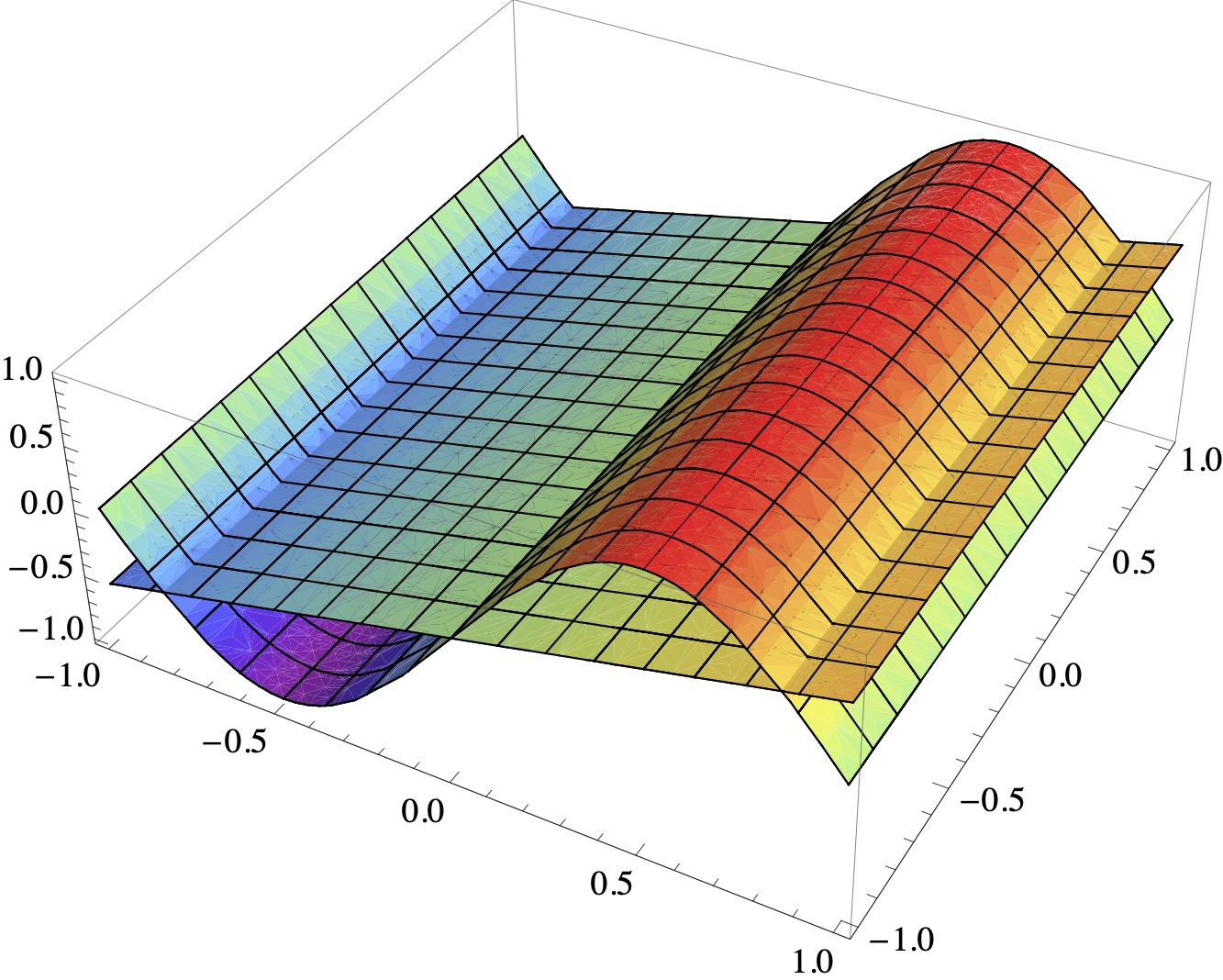
The right-hand side depends on \(v\). Choosing \(v(t_1,t_2) = \sin (\pi t_1)\) one obtains

\[\begin{split} \begin{align*} b_{00} &= \int_\Omega \sin (\pi t_1) \cdot 1 dt = 0,\\ b_{10} &= \int_\Omega \sin (\pi t_1) \cdot t_1 dt = \frac{\pi}{4},\\ b_{01} &= \int_\Omega \sin (\pi t_1) \cdot t_2 dt = 0. \end{align*} \end{split}\]

The resulting linear system is

\[\begin{split} \begin{align*} \begin{pmatrix} a_{00,00} & a_{00,10} & a_{00,01}\\ a_{10,00} & a_{10,10} & a_{10,01}\\ a_{01,00} & a_{01,10} & a_{01,01} \end{pmatrix} \begin{pmatrix} x_{00}\\ x_{10}\\ x_{01} \end{pmatrix} = \begin{pmatrix} 4 & 0 & 0\\ 0 & \frac{4}{3} & 0\\ 0 & 0 & \frac{4}{3} \end{pmatrix} \begin{pmatrix} x_{00}\\ x_{10}\\ x_{01} \end{pmatrix} = \begin{pmatrix} 0\\ \frac{\pi}{4}\\ 0 \end{pmatrix} = \begin{pmatrix} b_{00}\\ b_{10}\\ b_{01} \end{pmatrix}. \end{align*} \end{split}\]

The solution of the system is \((0,\frac{3 \pi}{16},0)\) and therefore the best approximation is

\[ p(t_1,t_2) =0 \cdot 1 + \frac{3 \pi}{16} \cdot t_1 +0 \cdot t_2 = \frac{3 \pi}{16} \, t_1. \]

The functions \(v\) and \(p\) are depicted here:

A remarkable feature of the example is that all off-diagonal entries in \(A\) vanish. This means that the basis functions are mutually orthogonal. In general, one cannot expect this. For instance, one can show that the functions

\[\begin{split} \begin{align} p_{00}(t_1,t_2) &= 1, &p_{01}(t_1,t_2) &= t_2, & p_{02}(t_1,t_2) &= t_2^2,\\ p_{10}(t_1,t_2) &= t_1, &p_{11}(t_1,t_2) &= t_1 \, t_2, & p_{12}(t_1,t_2) &= t_1 \, t_2^2,\\ p_{20}(t_1,t_2) &= t_1^2, &p_{21}(t_1,t_2) &= t_1^2 \, t_2, & p_{22}(t_1,t_2) &= t_1^2 \, t_2^2 \end{align} \end{split}\]

are a basis of \(\mathcal{Q}_{2,2} := \text{span}(p_{00}, \ldots, p_{22})\). Computing, for example,

\[ \langle p_{00}, p_{20} \rangle_{\Omega} = \int_\Omega 1 \cdot t_1^2 dt = \frac{4}{3} \]

implies that orthogonality is lost and that the matrix \(A\), implementing \(L^2\) approximation in \(\mathcal{Q}_{2,2}\) with \(p_{00}, \ldots, p_{22}\) as underlying basis, has off-diagonal entries.

One can already observe in the 1-dimensional case that the basis of the approximation space \(P\) needs to be chosen carefully. For instance, if \(P = \mathcal{P}_n\) with basis \(1, t, t^2, \ldots, t^n\), then the resulting matrix \(A\) is poorly conditioned for larger and even moderate values of \(n\). However, the `more orthogonal’ the basis functions are, the better conditioned the linear system is. In the ideal case, the basis is orthonormal, implying that \(A = I\).

There are different options to obtain an orthonormal basis in multivariate space. One can use the Gram-Schmidt method, which works for all (finite-dimensional) inner product spaces. For instance, one can start with the above \(p_{00}, \ldots, p_{22}\) to generate an orthonormal basis of \(\mathcal{Q}_{2,2}\) with this method.

However, assembling the multivariate basis from an orthonormal \(1\)-variate basis is often more economical. Let \(p_\alpha, p_\beta\) be orthogonal functions in \(L^2_\gamma((a,b),\mathbb{K}^m)\). Then the functions

\[ \begin{align} p_\alpha(t_1) \, p_\alpha(t_2), \quad p_\alpha(t_1) \, p_\beta(t_2), \quad p_\beta(t_1) \, p_\alpha(t_2), \quad p_\beta(t_1) \, p_\beta(t_2) \end{align} \]

are orthogonal in \(L_\eta^2((a,b)^2, \mathbb{K}^m)\) with \(\eta(t_1,t_2) = \gamma(t_1) \cdot \gamma(t_2)\) because

\[\begin{split} \begin{align} \langle p_j \, p_\ell, p_i \, p_k \rangle_{\Omega, \eta} &= \int_a^b \int_a^b \bigl( p_j(t_1) \, p_\ell(t_2) \bigr) \cdot \overline{\bigl( p_i(t_1) \, p_k(t_2) \bigr)} \bigl( \gamma(t_1) \, \gamma(t_2)\bigr) dt_1 dt_2\\ \label{eqn:prod_basis_argument} &= \int_a^b p_j(t_1) \cdot \overline{p_i(t_1)} \, \gamma(t_1) dt_1 \int_a^b p_\ell(t_2) \cdot \overline{p_k(t_2)} \, \gamma(t_2) dt_2\\ \nonumber &= \langle p_j, p_i \rangle_{(a,b), \gamma} \, \langle p_\ell, p_k \rangle_{(a,b), \gamma}\\ \nonumber &= \begin{cases} \| p_j \|^2 \cdot \| p_\ell \|^2 &: \mbox{ if $j=i$ and $\ell = k$}\\ 0 &: \mbox{ if $j\neq i$ or $\ell \neq k$} \end{cases} \nonumber \end{align} \end{split}\]

with \(i, j, k, \ell \in \{ \alpha, \beta \}\). In particular, if \(p_\alpha\) and \(p_\beta\) are orthonormal, then the products \(p_\alpha \cdot p_\beta\) are orthonormal.

Let us use this argument to construct an orthogonal basis of \(\mathcal{Q}_{2,2}\). Functions in \(\mathcal{Q}_{2,2}\) have the form

\[ \begin{align} p(t_1, t_2) = \sum_{j=0}^2 \sum_{k=0}^2 \alpha_{jk} t_1^j t_2^k. \end{align} \]

Recall that the \(t_1^j t_2^k\) are a basis of \(\mathcal{Q}_{2,2}\). Even without the proof that they are, in fact, a basis (which was omitted), one can directly conclude that \(\mathcal{Q}_{2,2}\) spanned by the \(9\) functions \(t_1^j t_2^k\), which means that \(\mathcal{Q}_{2,2}\) can at most be \(9\) dimensional.

We leave it as an exercise to check that the so-called Legendre polynomials

\[ L_0(t) = 1, \quad L_1(t) = t, \quad L_2(t) = \frac{3}{2} t^2 - \frac{1}{2} \]

are orthogonal in \(L^2((-1,1), \mathbb{R})\). Consequently, the functions

\[ p_{jk}(t_1, t_2) := L_j(t_1) \cdot L_k(t_2), \qquad j,k \in \{ 0, 1, 2 \}, \]

are orthogonal in \(L^2((-1,1)^2, \mathbb{R})\).

Fact: Independence of orthogonal vectors

Mutually orthogonal vectors in an inner product space \((V, \langle \cdot, \cdot \rangle)\) are linearly independent.

Thus, the \(p_{jk}\) are linearly independent. Moreover, the \(p_{jk}\) belong to \(\mathcal{Q}_{2,2}\). For instance,

\[ p_{1,2} = t_1 \cdot \Bigl( \frac{3}{2} t_2^2 - \frac{1}{2} \Bigr) = \alpha_{1,2} t_1 \, t_2^2 + \alpha_{0,0} t_1^0 t_2^0 \]

has the structure a linear combination in the original span with \(\alpha_{1,2} = \frac{3}{2}\) and \(\alpha_{0,0} = -\frac{1}{2}\).

Fact: Basis of orthogonal vectors

A selection of \(n\) linearly independent, nonzero vectors in an \(n\)-dimensional vector space \(V\), \(n \in \mathbb{N}\), is a basis of ,\(V\).

Therefore the \(p_{jk}\) are a basis of \(\mathcal{Q}_{2,2}\). The matrix \(A\) above is diagonal if the \(p_{jk}\) are orthogonal.

Example 3

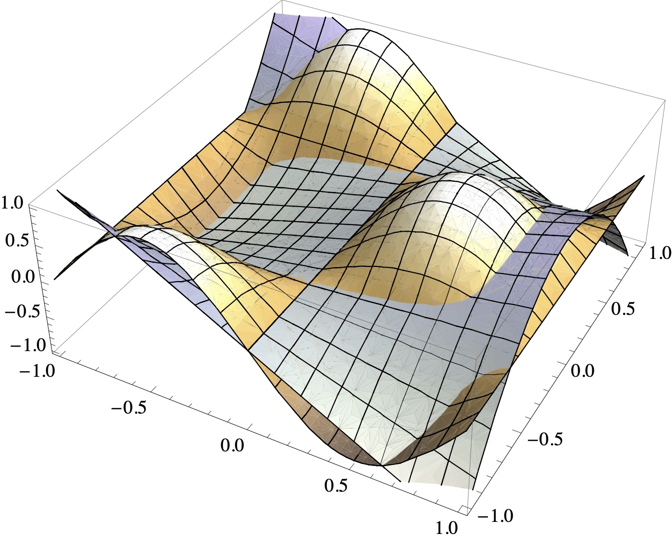
Let \(V = L^2((-1,1)^2, \mathbb{R})\). Compute the best approximation \(p\) to

\[ v(t_1, t_2) = \sin(\pi t_1) \, \cos(\pi t_2) \]

in \(P = \mathcal{Q}_{2,2}\).

We use the Legendre product basis for the computation. Then the coefficients \(\hat{x}_{jk}\) in

\[ p(t_1, t_2) = \sum_{j=0}^2 \sum_{k=0}^2 \hat{x}_{jk} p_{jk}(t_1, t_2) = \sum_{j=0}^2 \sum_{k=0}^2 \hat{x}_{jk} L_j(t_1) \cdot L_k(t_2) \]

are given by

\[\begin{split} \begin{align} \label{eqn:Lt_approx_example} \langle p_{jk}, p_{jk} \rangle_{(-1,1)^2} \, \hat{x}_{jk} & = \langle v, p_{jk} \rangle_{(-1,1)^2}\\ \nonumber & = \int_{-1}^1 \int_{-1}^1 \, \sin(\pi t_1) \, \cos(\pi t_1) L_j(t_1) \, L_k(t_2) dt_1 dt_2\\ \nonumber & = \int_{-1}^1 \sin(\pi t_1) \, L_j(t_1) dt_1 \; \int_{-1}^1 \cos(\pi t_2) \, L_k(t_2) dt_2, \end{align} \end{split}\]

taking the diagonal structure of the system into account. One calculates

\[\begin{split} \begin{align*} \int_{-1}^1 \sin(\pi t_1) \, L_0(t_1) dt_1 &= 0, & \int_{-1}^1 \cos(\pi t_2) \, L_0(t_2) dt_2 &= 0, \\ \int_{-1}^1 \sin(\pi t_1) \, L_1(t_1) dt_1 &= \frac{2}{\pi}, & \int_{-1}^1 \cos(\pi t_2) \, L_1(t_2) dt_2 &= 0,\\ \int_{-1}^1 \sin(\pi t_1) \, L_2(t_1) dt_1 &= 0,& \int_{-1}^1 \cos(\pi t_2) \, L_2(t_2) dt_2 &= - \frac{6}{\pi^2}. \end{align*} \end{split}\]

Therefore, the system of equations turns into

\[\begin{split} \langle p_{jk}, p_{jk} \rangle_{(-1,1)^2} \, \hat{x}_{jk} = \begin{cases} - \frac{12}{\pi^3} & \mbox{ if $j = 1$ and $k = 2$,}\\ 0 & \mbox{ if $j \neq 1$ or $k \neq 2$.} \end{cases} \end{split}\]

Furthermore,

\[ \langle p_{1,2}, p_{1,2} \rangle_{(-1,1)^2} = \int_{-1}^1 \int_{-1}^1 \Bigl( t_1 \cdot \Bigl( \frac{3}{2} t_2^2 - \frac{1}{2} \Bigr) \Bigr)^2 dt_1 dt_2 = \frac{4}{15}.\]

Therefore

\[ p(t_1, t_2) = \frac{15}{4} \Bigl( - \frac{12}{\pi^3} \Bigr) \; t_1 \; \Bigl( \frac{3}{2} t_2^2 - \frac{1}{2} \Bigr). \]